Data Structure Basics pt.5
Table of Contents
Tree Data Structures
The idea of a tree data structure, in its most generic sense, is that we have a collection of nodes that have one or more links connecting them to each other.
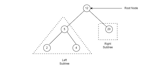
Tree data structures have a starting node, the root node. This node, like any other, can hold an object and links to its child nodes. The root node is their parent node. In fact, other than the root node, all nodes can be both parent and child nodes. Nodes that share the same parent node are siblings, and those that have no child nodes are called leaf nodes.
Binary Search Tree
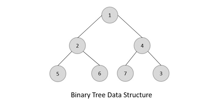
In a binary tree there can’t be more than two child nodes per parent node. They are called left child and right child nodes. The naming of these two nodes is quite relevant. The left child must be less than its parent. While the right one must be greater than it. We must make sure to follow this rule in order to keep the binary tree sorted so we can easily retrieve the objects in it.
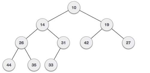
Simply adding data in the manner described above may lead to unbalanced BSTs; with more objects on one side than on the other. The disadvantage is that it would take longer to search for those objects on the busy side of our BST. Depending on how a BST is implemented it could reorganize itself if it becomes unbalanced.
Binary search trees often use key-value structures, like associative arrays, behind the scene. The key gets stored, together with the links to other nodes, directly in a node making it fast at insertion and retrieval. Due to being an ordered data structure it is possible to iterate sequentially through its nodes.
Binary Search Tress in Ruby
Ruby has no implementation of binary search trees.
Heaps
Heaps are typically used in sorting algorithms. But they are also a way of implementing other abstract data types, like priority keys. Heaps are usually implemented as binary trees (not to be confused with a BST); a collection of parent/child nodes with a maximum of 2 children an one parent. The difference is that we fill heaps from root to leafs, every pair of children is always filled from left to right before moving to fill the left node’s children. This way we don’t have to worry about the tree being unbalanced.
Even though a heap sorts itself every time a node is added or removed is not a fully sorted data structure. That’s because its nodes aren’t in a particular order, they’re just either lower or higher than their parent node. This means that a heap is not for retrieving but for keeping track of either the highest or lowest node. For that reason we might want to look into heaps when dealing with priority queues.
As mentioned before, there are two ways to fill in a heap. Which way to implement depends on whether we want to create a Min Heap or a Max Heap. That is, do we want the root node to contain the lowest or highest value?
Max Heaps
In Max Heaps child nodes must be less than their parent.
Min Heaps
If we want a Min Heap then child nodes must be greater than their parent.
Heaps in Ruby
Ruby has no implementation of heaps.
Introduction to Graphs
So far we’ve talked about a few data structures that deal with collections of nodes rather than objects/values, for instance, linked lists and heaps. All of them had distinct rules for connecting with other nodes. Graphs, on the other hand, is a collection of nodes where any node can connect with any other node. Also, it can connected to more than one node. The point of this kind of data structure is that there are no first or last nodes. So graphs are great when we need to describe a complex system of interconnected nodes.
Since graphs are closely related to graph theory in mathematics, is not uncommon to read about vertices (singular: vertex), meaning nodes, and edges (the connections between them). So a graphs is a set of vertices and edges.
Directed/Undirected Graphs
A directed graph is one whose edges only have one way. Edges in undirected graphs allow us to go in any direction.
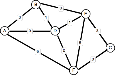
Weighted Graphs
If it is useful, we can give each edge a weight. This usually means labeling each edge with an integer. This could be useful if, for example, we want to figure out the shortest trip from one city to another by looking at the edges and figuring out the shortest option (assuming the edges labels represent the actual distance between the vertices it connects).
Next time
In the last part of the series we’ll check the main strengths and weaknesses of all the data structures we talked about. Until then, happy coding.